In the previous part of this project, we scraped the California Common Surgeries website and stored the data into a SQLite database. In this part, I will show how to do some simple but useful visualizations with the data using Google's Charts API.
We'll again be practicing SQLite queries. From the resulting data, we will then print out the necessary HTML to make web-ready graphics.
Hacking Visualizations
Ruby isn't particularly great for doing data visualizations. But just as we used SQLite to handle data, we can hook Ruby up with an external visualization library and quickly generate useful graphics.
For this chapter, I've chosen the Google Charts API because it's fairly easy to use, has a lot of flexibility, and simplifies bringing the visualizations to the Web; in fact, the graphics live on Google's server, so you can share and link to them easily.
If you had trouble creating the database from the last chapter, you can download a copy of the data I compiled here (includes both SQLite and plaintext).
Intro to the Google Charts API
Google already has a good tutorial on using their API. Here's the gist of how it works: you supply the data in the proper format. Google gives you a URL to an image you can view in your browser.
For example, here's the code to make a 300x100 pixel bar chart with values at 10, 40, and 80:
https://chart.googleapis.com/chart?cht=bhs&chs=300x200&chd=t:10,40,80
Click on that URL and you should see:
By now you should be familiar with web APIs and the syntax of URL parameter pairs with ? and &. The chs parameter refers to the chart size, as its value is 300x100. The chd parameter takes in data points in the form of t:10,40,80. And the first parameter, cht, has a value of bhs, which, after some reading of the API docs, we can take a guess that it stands for bar horizontal stacked.
Explore the API some more on your own. It's pretty self-explanatory.
Here's how to make a pie-chart that is 200x200 with wedges of 10, 20, 30 and 50:
https://chart.googleapis.com/chart?cht=p&chs=200x200&chd=t:10,20,30,50
You can add labels to correspond to each datapoint like so:
https://chart.googleapis.com/chart?cht=p&chs=300x150&chd=t:10,20,30,50&chl=Jan|Feb|Mar|Apr
And here's a line chart with two series of data. Notice how the chd parameter uses the pipe character | to separate the two data series:
Charts with Ruby
So what does this have to do with Ruby?
Well, for one, we can use loops to quickly output the image code.
For example, consider the famous Fibonacci sequence – which has implications far outside of mathematics, including the Golden Ratio used in the arts to how a plant's leaves are arranged – in which each number in the sequence consists of the sum of the previous two numbers:
1,1,2,3,5,8,13...
The Ruby code to generate the first 12 numbers and insert them into the API call to make a Google bar graph:
fibs = 11.times.inject([0,1]){|arr, num| arr << arr[-2] + arr[-1] }
imgstr = "http://chart.googleapis.com/chart?cht=bvs&chds=a&chs=400x250&chd=t:#{fibs.join(',')}"

puts imgstr
#=>   http://chart.googleapis.com/chart?cht=bvs&chds=a&chs=400x250&chd=t:0,1,1,2,3,5,8,13,21,34,55,89,144
There's one optional parameter I've included here: chds=a. By default, the Google API will scale the chart so that 100 is the maximum value. Without setting the chds parameter to a – which scales the chart according to the actual data – the 144 datapoint would be cut off.
Draw a stock prices chart
Of course, it's more fun to draw charts with dynamic data. Yahoo provides a nice API for daily stock numbers. Here's the URL for Xerox's stock price at the beginning of each month from 2007 to 2011:
http://ichart.finance.yahoo.com/table.csv?s=XRX&d=11&e=18&f=2011&g=m&a=1&b=11&c=2007&ignore=.csv
The data comes in this format:
Date,Open,High,Low,Close,Volume,Adj Close
2011-11-01,8.03,8.55,7.90,8.21,14545900,8.21
2011-10-03,6.80,8.65,6.55,8.18,17206800,8.18
2011-09-01,8.35,8.42,6.96,6.97,15507200,6.97
2011-08-01,9.49,9.53,7.30,8.30,21601000,8.25
Here's a sample data file if the Yahoo's API isn't working. Now it's a simple matter of fetching, parsing, and tacking the data onto Google's API for line charts.
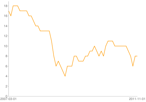
Here's how to graph the closing stock price: Since the CSV file is in reverse-chronological order, we have to reverse the datafile and also exclude the column headers. I also include the necessary parameters in Google's API to label the axes.
One more thing: You can't send the Google API a URL longer than 2,000 characters. So to be safe, I've limited the data to 100 rows and I've rounded the prices to dollars using to_i:
Here's what the URL looks like:
https://chart.googleapis.com/chart?cht=lc&chs=500x350&chds=a&chxt=x,y&chxl=0:|2007-03-01|2011-11-01&chd=t:17,16,18,18,18,17,17,17,17,16,16,15,14,14,13,13,13,13,13,11,8,6,7,6,5,4,6,6,6,8,8,7,7,7,8,8,9,9,10,9,8,9,8,10,11,11,11,10,10,10,10,10,10,9,8,6,8,8
And the resulting image:
For the remainder of this chapter, the charts won't get much more complicated. It's worth browsing the detailed chart API docs, though, just to see all the available possibilities.
Queries and graphing
This next section will contain a combination of SQLite queries, iterating through the resulting arrays of data, and printing out the appropriate Google Charts API code.
Here's the setup based on what we did in the previous chapter of this project:
require 'rubygems'
require 'sqlite3'

DBNAME = "data-hold/ca-common-surgeries.sqlite"
DB = SQLite3::Database.open( DBNAME )
TABLE_NAME = "surgery_records"
The rest of the code examples in this book depend on the above variables being set.
Number of discharges per procedure
Let's start with a simple graphic: Sum the number of discharges per procedure in the database. Create a horizontal bar chart with labels.
The SQLite query:
q = "SELECT procedure, SUM(discharge_count)
   FROM #{TABLE_NAME}
   GROUP BY procedure
   ORDER by procedure DESC"

results = DB.execute(q)
Now iterate through the array of results. Note that I select an abbreviation of the procedure names to fit them on the chart.
procedures = results.map{|row| row[0].split(' ').map{|s| s[0..3]}[0..2].join.gsub(/[^\w]/,'')}
discharge_counts = results.map{|row| row[1]}
G_URL = "https://chart.googleapis.com/chart?cht=bhs&chs=400x600&chds=a&chbh=10&chxt=x,y"
puts "#{G_URL}&chd=t:#{discharge_counts.join(',')}&chxl=1:|#{procedures.join('|')}"
– which results in this massive URL:
https://chart.googleapis.com/chart?cht=bhs&chs=400x600&chds=a&chbh=10&chxt=x,y&chd=t:11991,7085,10376,17159,2481,79173,5879,3911,4888,21269,4381,44201,14711,3085,7655,131252,3559,220,27745,14843,73431,13970,65393,15147,1819,28123,3654,19555,4161,18226,26842,27080,7315,15675,221401,178462,1478&chxl=1:|TotaRemoof|Thyruni|Thyrtot|TURPTran|TULILase|SpinFusiany|ShouRepltot|ShouReplpar|RepaUrinStre|RadiPros|Para|PTCACorAngi|Mastuni|Mastbil|LapBandins|KneeRepltot|InguHernRepa|InguHernRepa|HystVagi|HystVagi|HystAbdo|HystAbdo|HipRepltot|HearValvRepl|GastBypaope|GastBypalap|GallRemoope|GallRemolap|EndoRemoof|EndaRemof|DiscRemoany|ColeLargInte|ColeLargInte|CABGCorArte|CSeDeli|AssiVagiDeli|AbdoProsret
Median cost of procedure per hospital over time
For all Sacramento County hospitals, show the median cost of Disc Removal (any level) procedures over 2007 to 2009. As I mentioned at the beginning of the project, the OSHPD states that some hospitals do not report median charge data. So add a condition to only include rows where median_charge_per_stay is greater than 0.
SQL subqueries
I wrote this section before deciding to write an entire chapter on SQL. You may find that explanations there more helpful than here.
Prepare for some convoluted SQL...
Here's the query:
SELECT s.hospital,
(SELECT s2007.median_charge_per_stay FROM surgery_records AS s2007
   WHERE s2007.hospital=s.hospital AND s2007.county=s.county
   AND s.procedure=s2007.procedure AND s2007.year=2007) AS mc2007,
(SELECT s2008.median_charge_per_stay FROM surgery_records AS s2008
   WHERE s2008.hospital=s.hospital AND s2008.county=s.county
   AND s.procedure=s2008.procedure AND s2008.year=2008) AS mc2008,
(SELECT s2009.median_charge_per_stay FROM surgery_records AS s2009
   WHERE s2009.hospital=s.hospital AND s2009.county=s.county
   AND s.procedure=s2009.procedure AND s2009.year=2009) AS mc2009

FROM surgery_records AS s
WHERE s.county='Sacramento'
   AND s.procedure='Disc Removal (any level)'
   AND s.median_charge_per_stay > 0
GROUP BY s.hospital
ORDER by s.hospital, s.year ASC
If you're new to SQL, that multi-line query may be intimidating. Let me reduce it to something more familiar:
q = "
SELECT s.hospital,
mc2007, mc2008, mc2009
FROM surgery_records AS s
...
Where do the columns mc2007, mc2008, mc2009 come from? They're the result of subqueries (that I've omitted in the code right above). Think about what datapoints we're looking for: the median charge of a particular operation for a particular hospital for a given year.
We don't have a column for median_charge_per_stay in 2007. We have a columns for year for median_charge_per_stay. By using a subquery, we're able to create a new column of data for our results set.
Here's one of the subqueries:
SELECT s2007.median_charge_per_stay FROM surgery_records AS s2007
   WHERE s2007.hospital=s.hospital AND s2007.county=s.county
   AND s.procedure=s2007.procedure AND s2007.year=2007
This uses table aliasing. When using a subquery upon the same table as our main query (surgery_records), SQLite essentially does a query on a copy of that table. So we need to give each instance of the table an alias:
SELECT s2007.median_charge_per_stay FROM surgery_records AS s2007
This SELECT statement is acting on a version of surgery_records that I've arbitrarily named as "s2007". You can name it anything, generally, you want to give it a shorter name than the original table to save yourself some typing.
From the table now known as s2007, we want to select the median_charge_per_stay. However, since there will be multiple tables – including the table accessed in the main query – with the column median_charge_per_stay. So we specify that we want the version found in s2007, thus: s2007.median_charge_per_stay
Where does the subquery fit into the main query? Just like any other column of data:
SELECT s.hospital,
      (SELECT s2007.median_charge_per_stay FROM surgery_records AS s2007
         WHERE s2007.hospital=s.hospital AND s2007.county=s.county) AS mc2007,
         ...
      FROM surgery_records AS s
Note that we have to give the subquery column a name (mc2007 – again, the name is of your choosing) and that we have aliased the surgery_records in the main query as s. This allows us to refer to the main query's version of the surgery_records inside the main query. This is, of course, the point of all this work: the main query is returning a list of hospitals (s.hospital) along with each hospital's yearly median_charge_per_stay. The subquery needs to know which record to compare against for its WHERE clause, e.g. WHERE s2007.hospital = s.hospital
If you mix up the aliases in the subqueries – e.g. s2007.hospital = s2008.hospital – the results will likely be erroneous.
One more thing: the subquery must return exactly one datapoint. Think about it: the main query's SELECT statement expects each column to have one datapoint per result row, just like a column in any regular spreadsheet. If the subquery returns several rows with several columns, well, that's not a single datapoint.
If our example subquery:
   ...
   (SELECT s2007.median_charge_per_stay
      FROM surgery_records AS s2007
      WHERE s2007.hospital=s.hospital AND s2007.county=s.county)
...
– returned more than one datapoint, then we've made the wrong assumptions about the data. We were expecting that each hospital had exactly one record per procedure per year.
Back to the code
Using a Ruby loop and string interpolation, we can save ourselves from typing that entire tedious query:
q = "SELECT s.hospital,
#{
   [2007,2008,2009].map{ |yr|
      "(SELECT s#{yr}.median_charge_per_stay FROM #{TABLE_NAME} AS s#{yr} WHERE s#{yr}.county=s.county AND s#{yr}.procedure=s.procedure AND s#{yr}.hospital=s.hospital AND s#{yr}.year=#{yr}) AS mc#{yr}"
   }.join(",\n")
}
FROM surgery_records AS s
WHERE s.county='Sacramento'
   AND s.procedure='Disc Removal (any level)'
   AND s.median_charge_per_stay > 0
GROUP BY s.hospital
ORDER by s.hospital, s.year ASC"
If you were to run that query in a GUI like Firefox's SQLite manager (after resolving all the variable names and string interpolation, of course), this is what the data looks like:
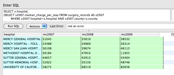
And in Ruby array form:
results = [
   ["MERCY GENERAL HOSPITAL","31045","35610","38532"],
   ["MERCY HOSPITAL - FOLSOM","23488","24669","26314"],
   ["MERCY SAN JUAN HOSPITAL","56108","39674","46115"],
   ["METHODIST HOSPITAL OF SACRAMENTO","39184","47653","11925"],
   ["SUTTER GENERAL HOSPITAL","44657","42913","43404"],
   ["SUTTER MEMORIAL HOSPITAL","52922","50150","48746"],
   ["UNIVERSITY OF CALIFORNIA DAVIS MEDICAL CENTER","58275","68519","82656"]
]
Remember that for a multi-series set of data, the Google API wants the data in this format:
&chd=t:x0,x1,x2|y0,y1,y2|z0,z1,z2
To generate that string with Ruby:
s2007 = results.map{|r| r[1]}.join(',')
s2008 = results.map{|r| r[2]}.join(',')
s2009 = results.map{|r| r[3]}.join(',')
chd = "&chd=t:" + [s2007,s2008,s2009].join('|')
puts chd
#=>    &chd=t:31045,23488,56108,39184,44657,52922,58275|35610,24669,39674,47653,42913,50150,68519|38532,26314,46115,11925,43404,48746,82656
Or, if you want to get fancier with your Enumerable-fu:
chd = "&chd=t:" + results.inject([]){ |arr, row|
   row[1..3].each_with_index{ |yr_pt, idx| arr[idx] ||= []; arr[idx] << yr_pt}
   arr
}.map{|a| a.join(',')}.join('|')
Tack that on to the appropriate Google API call for a vertical grouped-bar graph (I've omitted the hospital names as labels):
g_url = "https://chart.googleapis.com/chart?cht=bvg&chs=500x400&chds=a&chbh=5,2,10&chxt=y"
puts "#{g_url}#{chd}"
Scatterplot of procedure cost versus number of discharges and median length of stay
One of the things that stands out in the previous bar graph of disc removal surgeries in Sacramento County is the wide variance in median price per visit. In 2009, the Methodist Hospital of Sacramento median price was $11,925. UC-Davis, meanwhile, had a median price of $82,656.
Before jumping to any conclusions, let's consider the other variables: median length of stay and number of discharges.
Obviously, the number of days a patient stays in the hospital most likely has the strongest correlation. The latter may also have an impact in that a hospital may be a renowned specialist in a type of surgery, and thus may be able to perform with more efficacy, both in terms of patient outcomes and in cost.
Using Sacramento County again and focusing on the year 2009, we can get the necessary records with a simple query:
SELECT hospital, discharge_count, median_charge_per_stay, median_length_in_days FROM surgery_records
      WHERE county='Sacramento' AND procedure='Disc Removal (any level)' AND median_charge_per_stay > 0 AND year = 2009
      ORDER by hospital
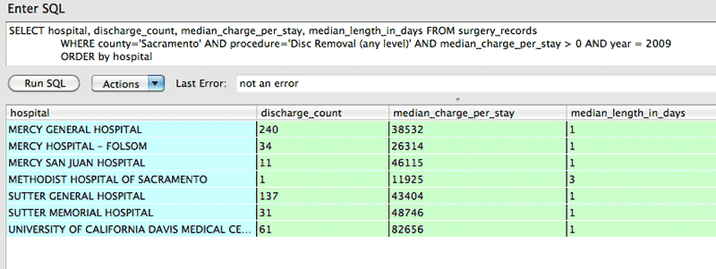
It looks like median_length_of_days only ranges from 1 to 3. Incidentally, the hospital with the lowest median charge, Methodist Hospital of Sacramento, is the only hospital that has more than 1 day as the median length of stay. It also had one discharge for this procedure, so it's not particularly of statistical interest.
So let's ignore median_length_of_days for now just do a simple scatterplot of discharge_count and median_charge_per_stay on the x- and y-axis, respectively. Here is how to form the Google API call for a scatterplot. Once again, we ignore the name of the hospitals for now in favor of seeing just the numbers:
q = "SELECT hospital, discharge_count, median_charge_per_stay
   FROM surgery_records
      WHERE county='Sacramento' AND procedure='Disc Removal (any level)' AND median_charge_per_stay > 0 AND year = 2009 AND discharge_count > 1
      ORDER by hospital"

chd = DB.execute(q).inject([[],[]]){ |arr, row|
   arr[0] << row[1]
   arr[1] << row[2]
   arr
}.map{|a| a.join(',')}.join('|')

g_url = "http://chart.googleapis.com/chart?cht=s&chs=500x300&chds=a&chxt=x,y&chd=t:#{chd}"
The URL:
http://chart.googleapis.com/chart?cht=s&chs=500x300&chds=a&chxt=x,y&chd=t:240,34,11,137,31,61|38532,26314,46115,43404,48746,82656
The resulting image is less than compelling:
There doesn't appear to be a strong correlation between discharge_count and the median_charge_per_stay in Sacramento hospitals, as hospitals vary wildly in both.
All counties, all procedures, for 2009
What happens if we expand the query to include all counties? The number of datapoints would likely exceed the 2,000 character limit. So let's limit the query to include only 2009 records in which a hospital had more than 50 discharges for a given procedure.
And, for the hell of it, since this query is so simple, let's run it for each of the procedures – all 37 of them – and generate a web page so we can quickly glance at the scatter plots.
Nothing new here, just your regular HTML-string concatenation and writing to file:
require 'rubygems'
require 'sqlite3'
DBNAME = "data-hold/ca-common-surgeries.sqlite"
DB = SQLite3::Database.open( DBNAME )
TABLE_NAME = "surgery_records"
procedures = DB.execute("SELECT DISTINCT procedure from surgery_records")
q="SELECT hospital, discharge_count, median_charge_per_stay FROM surgery_records WHERE
discharge_count >= 25 AND median_charge_per_stay > 0 AND year = 2009 AND procedure=? ORDER by hospital"
outs = File.open("data-hold/procedures-all-hospitals-cost-vs-discharges.html", 'w')
outs.puts ""
procedures.each do |procedure|
chd = DB.execute(q, procedure).inject([[],[]]){ |arr, row|
arr[0] << row[1]
arr[1] << row[2]
arr
}.map{|a| a.join(',')}.join('|')
g_url = "http://chart.googleapis.com/chart?cht=s&chs=500x300&chds=a&chxt=x,y&chd=t:#{chd}"
outs.puts ""
end
outs.closeHere's a screenshot of the webpage that we just created (zoomed out to an illegible level):
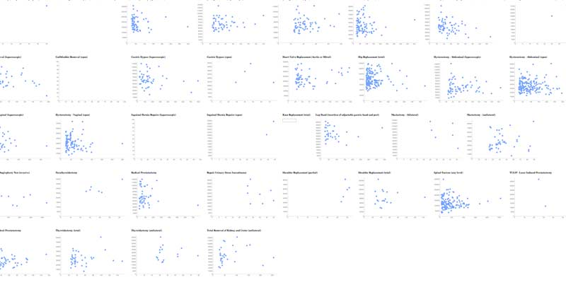
You can view the results here. Without getting into statistics, you can see that for some operations, there appears to be some correlation between hospitals' discharge counts and their median charges for a given procedure, e.g. the more times a hospital does a procedure, the lower they keep the costs.
This could possibly describe the scatterplot for gastric bypass (laparoscopic):
However, there are operations for which the opposite is true. Look at mastectomies (unilateral):
How can this have the opposite correlation from what we saw with gastric bypass surgeries? Well, there are a number of factors that the data we have does not capture. It may be the case that the hospitals that with the best service and state-of-the-art technology – and thus, charge accordingly for it – also draw the most scheduled procedures.
What have we learned?
Given the caveats in the introduction, it's possible that none of my hypotheses are correct because the prices given are the full prices that a hospital lists, and not the actual amount received. That's a problem. But at least we've gained a little more insight to the strange system of medical pricing (if you weren't aware of it before).
Further avenues of research
And what about other factors, such as geography. These non-interactive Google charts don't make it easy to see which datapoint corresponds to which hospital, so we can't see whether location has any effect. Are there regions in which there is more of a correlation? Or, at least, less variance in median cost per procedure?
Those tangents are beyond the scope of this chapter, but hopefully I have given you enough examples so that you know where to start. Geographical information can easily be mashed into this project with Google's Geocoding API, which we covered briefly in Methods Part II
As I said in the introduction, this surgery-costs project was one of the first things I wrote when I started this book. Since then, I have drastically changed the roadmap, including writing a separate chapter for SQL, and so I've felt less compelled to fully flesh this project out.
There may be more to this data; I just haven't gotten around to it. But my caveats in the introduction still stand. And so any meaningful revelations from this data will require dedicated reporting and interviewing of hospital and state officials, because of some of the seemingly erratic results we've found so far.
Why coding makes data easier
If the crash course in SQL subqueries made you ill, keep in mind that it's just a matter of not letting large blocks of code intimidate you. When you break it down, the SQL commands are conceptually simple.
You can of course avoid using subqueries by depending more on Ruby loops to execute variations of the main query. But again, there's a tradeoff in readability and code complexity, which you'll appreciate if you ever have to revisit that code a month later.
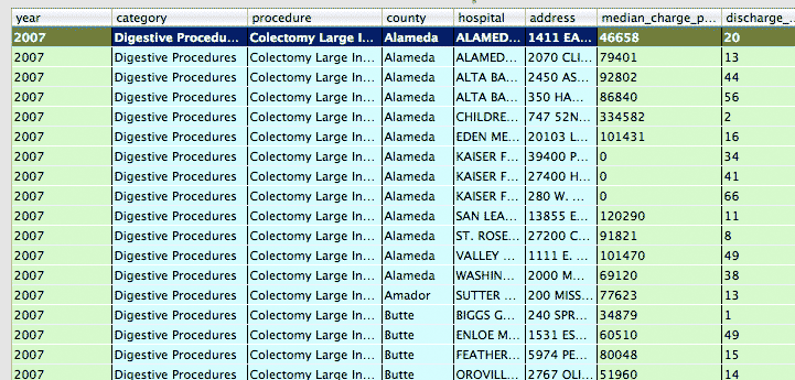
What about restructuring the entire table? Its current structure means that there is a row for every combination of hospital, year and procedure:
What if instead, we remove the year column and replace it with year_2007_median_charge, year_2008_median_charge, year_2009_median_charge, like so?
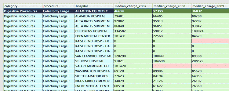
If all we needed to do was a single messy query, this might be the optimal solution. In fact, if you're sending the data to others who don't know SQL, it might be necessary to create these cost-by-year columns.
However, this means creating by-year columns for all the data points that are dependent on year, such as year_2007_median_length_in_days and year_2007_discharge_count.
And in the future, what if a 2010 set of data becomes available? Then you'll have to add new year_2010_... columns. In general, changing the column structure of the table is much more difficult than just adding rows of data.
Adding year_by columns makes the data easier for human readability because it's easier to scan and make comparisons across a single row than to do so across multiple rows. But there is a major penalty in the ability to maintain and to do automated queries in the future. For example, to do an average of year_x_median_charge columns, you would have to read the table structure and determine how many such columns exist.
This gets to the core of how programmers have an advantage over non-programmers. The latter are limited to simple single-row comparisons. But those who know code can do complex comparisons and tabulations on the fly, including generating those simple single-row comparisons for the non-programmers to read.
It takes work to gain this flexibility. But you'll come to appreciate the data-analyzing power you gain. And the time saved.