
SQL, short for Structured Query Language is a programming language for querying and managing databases. It has its own syntax and different database systems – including Microsoft Access, MySQL, PostgreSQL, and SQLite – all have their own variations of SQL.
I introduce SQL to acquaint you with databases in general, as they are essential to any serious kind of data-crunching/storing web application. Don't expect this to be an exhaustive reference of SQL. But you'll see how the Ruby language can be used to work with a completely different piece of software.
This section is entirely optional. But I will be using databases for most of the data-heavy projects that I plan to cover in this book. I provide an archetypical use-case with California's Commmon Surgeries database.
Fair warning: Even after a few years of dabbling with it, SQL syntax is still befuddling to me. And it might be the same for you, too. However, the power (and ubiquity) of SQL databases has so far surpassed my clumsiness in using it. I've found that the best way to learn is to think of the kinds of queries and aggregations that you might be able to do in Excel easily. And then look up how other programmers have written them up in SQL.
The best resource I have found on the web for SQL examples, by far, is from Artful Software Development, authors of "Get It Done With MySQL". Artful Software has generously created an online version of a chapter focusing on common queries: the result is a readable, gigantic list of virtually every query I have so far imagined.
Data-crunching without databases
Let's take a minute to step back and see how data programming might work without the use of a database. Included among the list of this book's projects is a stock market analysis which reads from a comma-delimited text file that contains the date and the Dow Jones index for that day.
You can easily create a Hash that holds the values, like so:
{:company=>"Acme Inc.", :ticker_symbol=>"ACME",
      :state=>"CA", :category=>"widgets", :date=>"8/1/2010",
      :closing_price=>"12.00"}
But things get unwieldy when dealing with data with multiple entries per entity:
[
   {:company=>"Acme Inc.", :ticker_symbol=>"ACME",
      :state=>"CA", :category=>"widgets", :date=>"8/3/2010",
      :closing_price=>"16.00"},
   {:company=>"Acme Inc.", :ticker_symbol=>"ACME",
      :state=>"CA", :category=>"widgets", :date=>"8/2/2010",
      :closing_price=>"14.00"},
   {:company=>"Acme Inc.", :ticker_symbol=>"ACME",
      :state=>"CA", :category=>"widgets", :date=>"8/1/2010",
      :closing_price=>"12.00"}
]
Such data can be expressed as a many-to-one relationship, in which there are many closing price records per company:
[{
    :company=>"Acme Inc.", :ticker_symbol=>"ACME",
    :state=>"CA", :category=>"Widgets",
    :closing_price_records=>
      [{:date=>"8/3/2010", :closing_price=>"16.00"},
       {:date=>"8/2/2010", :closing_price=>"14.00"},
       {:date=>"8/1/2010", :closing_price=>"12.00"}]
 },
 {
   :company=>"AppleSoft", :ticker_symbol=>"APLSFT",
   :state=>"TN", :category=>"Computers",
   :closing_price_records=>
       [{:date=>"8/3/2010", :closing_price=>"16.00"},
       {:date=>"8/2/2010", :closing_price=>"14.00"},
       {:date=>"8/1/2010", :closing_price=>"12.00"}]
}]
This data structure – an array of hashes, each of which contains company information, including an array of hashes of stock prices for that company – is not terribly difficult to work with for simple queries. For instance, to find all instances in which "Acme, Inc." had a closing price of less than $10, in the timeframe of 2009 to 2010, you might try:
   data.select{|c| c[:company] == "Acme Inc."}[0][:closing_price_records].select{ |r|
      r[:date] >= "2009" && r[:date] <= "2010" && r[:closing_price] < 10
   }
This query would obviously return funky results because I wrote out the examples using dates and amounts as strings instead of using the Date and number classes. But it's just pseudo-code, you get the picture...
Some coders may be more comfortable translating text files into Ruby data structures. But the reality is in the data-world is that you'll encounter many datasets that are either in a SQL format or are more easily stored as such. Database systems are also designed to handle massive datasets and to optimize complicated queries.
I learned some SQL before I knew Ruby just because I had to for my work, and so it's a habit for me to mix both languages in my scripts. But I really cannot argue that my workflow is a best practice or that it's worth your time to juggle two different languages. But I do believe that SQL and other database languages – as well as database design in general – is so ubiquitous that you need to pick up the knowledge at some point.
I only offer this chapter as a quick startup guide and demonstration of SQL in the context of Ruby programs. Thankfully, basic SQL queries are pretty easy to figure out for our purposes.
The project examining the cost of common surgeries in California has a section comparing the code for executing SQL queries versus iterating through a Ruby collection.
Getting started with SQLite
For the first part of this chapter, there won't be any Ruby coding. I'll walk you through how to setup SQLite on your system, how to work within its environment, and then introduce a series of example queries.
Database systems, like any other software, can be a bear to install. I choose SQLite because it is easy to install and requires comparatively little overhead.
Installation of SQlite
Mac OS X Leopard and after already have it pre-installed. Windows users may have to follow these steps:
- Go to the SQLite download page and look for the Precompiled Binaries For Windows section.
- Download two zip files: one for the shell and one for the DLL
- Unzip them in C:\Windows\System32. You may also/instead want to have these files in C:\ruby\bin (if you used the default settings for installing Ruby)
Again, my knowledge of software installation is mostly informed by Google and StackOverflow. If these instructions don't work, you may have to do some searching.
Running SQLite
If SQLite is correctly installed, you should be able to go to your command line and type: sqlite3
You should see something like this:
>> sqlite3 test.db
SQLite version 3.6.12
Enter ".help" for instructions
sqlite>
This is the SQLite interactive shell. You can type in SQLite commands just as you do in Ruby's irb.
There's one important and immediate syntax distinction. In Ruby, a line of code (as long as you aren't in the middle of a string, block, or parenthized expression) will execute when you hit Enter. In SQL, you need to end each statement with a semi-colon ;
Here's a "Hello world" statement to see if everything is working:
sqlite> select "hello world";
hello world
Using Firefox as a SQLite interface
If you haven't already, I recommend installing the Firefox browser. Not only is it a good browser, but it has many plugins that are useful (and free) tools for every programmer.
Firefox uses SQLite to store browsing history so the user "lazierthanthou" has created a plugin – SQLite Manager – that serves as a convenient graphical user interface for exploring SQL and database files.
For the screenshots in this example, I will be using SQLite Manager. You can download it here.
A sample database of stock prices
For the purposes of this chapter, I've created a database of the S&P 500 companies and their historical stock prices, using the listing at Wikipedia and the Yahoo API.
Download it here: sp-500-historical-stock-prices.zip
Unzip the file in a directory. The name of the file should be: sp500-data.sqlite
After you've downloaded SQLite Manager, open up the Firefox browser and go to the Tools submenu:
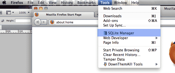
Click on the SQLite Manager item. This should pop up a new program window that looks like this:

Click on the Open icon (circled in red) and select the sp500-data.sqlite file.
In the left side of the SQLite Manager window should be a list of submenus relating to the sp500-data.sqlite database file. Select Tables and then `companies`.
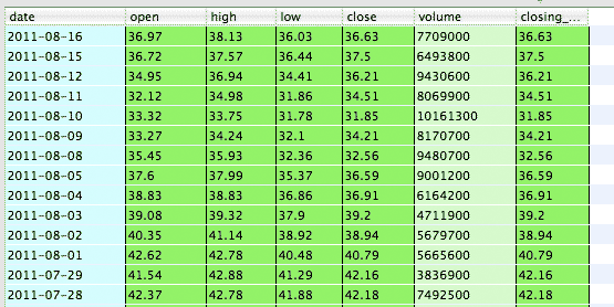
Then in the row of non-icon buttons near the top, select Browse & Search:
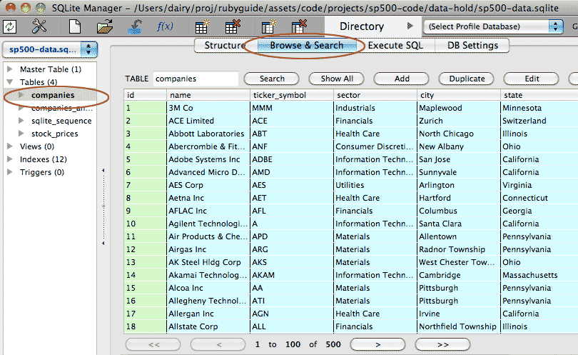
In this view, you have a spreadsheet-like view of each data table. This is nice for reminding yourself what the table looks like. But you typically won't be using this view to search for data.
Write your first query
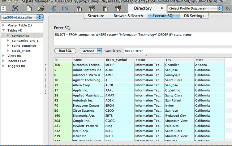
In the top row of text-buttons, click Execute SQL. This is where you write raw SQL queries.
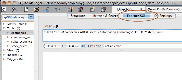
Let's write a query to list tech companies and order them by state. In the text box labeled Enter SQL, type the following and click: Run SQL
SELECT * FROM companies WHERE sector="Information Technology" ORDER BY state, name
A spreadsheet-like listing should appear at the bottom. It will look similar to the Browse & Search view. The difference is that our custom query generated this listing.
For the next section on SQL syntax, this is where we will be practicing our queries.
SQL syntax
The best way to approach SQL language is to think of that S in its name: Structured
Early on, you're going to get a lot of error messages as you try to figure out the proper order of a SQL statement, but at least there's a (usually) consistent pattern to memorize.
We'll start with the simplest building block of a statement and gradually add on to it.
You can practice this next section in any SQL environment you like. Again, I'll be using Firefox's SQLite plugin, but anything that allows you to open up a SQLite database and type in SQLite commands will suffice.
We will not be writing any Ruby code during this exploration of the SQL basics.
The SELECT
Most of the SQL statements involve selecting records from the database. The SQL syntax for that is: SELECT.
Besides retrieving rows from the database, the SELECT can be asked to select literal values, such as numbers and strings.
SELECT takes a list of values or names of tables and columns, separated by commas.
The following will return one record with two columns, one for each string:
SELECT "Hello world", "And this is another string";
A couple of syntax things:
- Capitalization usually doesn't matter. However, I will try to put SQL-specific syntax in all-uppercase for easier reading.
- End each command with a semi-colon.
The FROM
In order to SELECT records from our database, we have to specify the name of the target table. This is done with FROM.
To select all columns from a table, we SELECT the asterisk operator *
SELECT * FROM companies_and_stocks
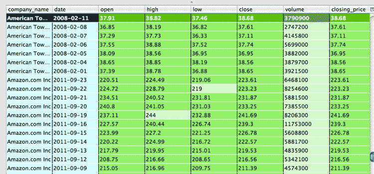
From our sample database, we should get about 30,000* rows with all the columns from companies_and_stocks. With the Firefox plugin, it should look like this:
* in the companies_and_stocks table, only records in the most recent couple of months are included. The other tables have the full set of data.
We can also select specific columns of a table:
SELECT companies_and_stocks.name, companies_and_stocks.date,
   companies_and_stocks.closing_price FROM companies_and_stocks
The dot operator denotes that name, date and closing_price belong to companies_and_stocks. Specifying the table name is optional unless more than one table in your database has a column with the given name.
And you don't have to select only columns. You can SELECT calculations based on values in a column. The following command selects several columns and a column consisting of the closing_price values multiplied by 10. The values in name and ticker_symbol are converted to uppercase and lowercase characters, respectively:
SELECT  UPPER(name),
      LOWER(ticker_symbol),
      10 * closing_price
      FROM companies_and_stocks;
Note that whitespace is not significant in MySQL, just like in Ruby. You can use line-breaks and tabs to make a query more readable.
The WHERE
Getting back every row from a data table isn't always necessary or useful. So to filter the results, we use the WHERE keyword to specify conditions, such as: "return the rows where the amount is greater than 42".
Comparison and logical operators
The comparison operators – <, >, <=, != and so forth – are the same as in Ruby. However, the equality operator uses just a single =
Logical operators are written out: AND instead of &&, OR instead of ||.
| Operation | Ruby | SQL |
|---|---|---|
| Equal to |
==
|
=
|
| Not equal to |
!=
|
!=
|
| ... and ... |
&&
|
AND
|
| ... or ... |
||
|
OR
|
The following code would fetch all rows where closing_price is between 100 and 200:
SELECT * FROM companies_and_stocks WHERE closing_price > 100 AND closing_price < 200;
The WHERE conditions can get as complex as you want, including the use of a series of logical operators and parentheses to specify order of comparisons:
SELECT * FROM companies_and_stocks WHERE
   (closing_price > 100 AND closing_price < 200)
   OR (sector = 'Financials' AND closing_price > 200);
SELECT * FROM companies_and_stocks
WHERE closing_price > 100 AND
closing_price < 200 OR sector = 'Financials' AND closing_price > 200;
The difference between the above queries (remember that whitespace doesn't matter) is that the first query will fetch rows where closing_price is between 100 and 200 OR if sector has a string value equal to 'Financials' while having a closing_price value greater than 200.
The second query, without the parentheses, will return nothing, because the final AND'ed condition – closing_price > 200 – will never be trueif the first two conditions – closing_price is more than 100 and less than 200 – is also true.
Using strings
As in Ruby, SQL treats strings differently than numbers. Strings must be enclosed in single or double quote marks:
SELECT * FROM companies_and_stocks WHERE ticker_symbol="TXN"
In the sample database, all the data is free of double-quote marks. So use those to avoid erroneously quoted queries such as:
SELECT * FROM companies_and_stocks WHERE name='John's Apples'
How to get hacked
The following is just a segue on database security and doesn't apply to what we're working on now.
Remember in Ruby how not properly closing strings off with quote marks led to some annoying errors? In SQL-Land, such errors allow for the most easily performed yet catastrophic technique for hacking websites and databases.
The hack occurs anytime a website or program takes in input from the user without sanitizing it. Imagine that a website allows the user to enter stock symbols. The website then connects to the database with the following query and inserts the user's input in between the quote marks:
SELECT * FROM companies_and_stocks WHERE ticker_symbol=""
But instead of entering a stock symbol, the user types quotation marks – and some evil SQL code. Below is the original query with the user's malicious input highlighted in red:
SELECT * from companies_and_stocks WHERE ticker_symbol="whatev";
   DROP TABLE companies_and_stocks; SELECT "Ha ha!"
(Don't run the above script unless you want to redownload the sample database)
This is called SQL injection and is easily prevented. In this case, the sanitizing involves inserting escaping backslashes in front of every quotation mark from the user:
SELECT * from companies_and_stocks WHERE ticker_symbol="whatev\";
   DROP TABLE companies_and_stocks; SELECT \"Ha ha!"
The query ends up being a harmless (and fruitless) search for a ticker_symbol equal to whatev\"; DROP TABLE...
Most scripting languages have libraries that handle this easily. And yet SQL injections continue to result in spectacular hacking attacks.
Just something to put on your checklist before you start building your first database-backed website...However, the SQLite3 gem has a convenient method for handling the proper quoting of input, which I cover in the section about placeholders.
Fuzzy matching with LIKE
The LIKE keyword allows you to do partial matching of text values. By default, it matches values without regard to capitalization. So instead of:
SELECT * FROM companies_and_stocks WHERE name = 'V.F. Corp.' OR name = 'V.F. CORP.';
The use of LIKE will capture all variations of capitalization:
SELECT * FROM companies_and_stocks WHERE name LIKE 'V.F. CORP.';
The percentage sign %, when used as part of a string value, serves as a wildcard. The following three statements select rows in which name starts with 'Ba' (again, case-insensitive), ends with 'co', or contains the characters 'oo' somewhere:
SELECT * FROM  companies_and_stocks WHERE name LIKE 'Ba%';
SELECT * FROM  companies_and_stocks WHERE name LIKE '%co';
SELECT * FROM  companies_and_stocks WHERE name LIKE '%oo%';
ORDER BY
The result set can be sorted with the ORDER BY syntax, followed by a column name:
SELECT * FROM companies_and_stocks WHERE name LIKE 'Ba%' ORDER BY closing_price;
You can sort by more than one column. The first listed column will have the most priority:
SELECT * FROM companies_and_stocks WHERE name LIKE 'Ba%' ORDER BY state, closing_price;
The sort order can be specified with the ASC – ascending order is the default – and DESC keywords:
SELECT * FROM companies_and_stocks WHERE name LIKE 'Ba%' ORDER BY state ASC, closing_price DESC;
LIMIT
This is often the last keyword in a SELECT statement. It limits the number of rows returned, which is useful in cases where you might just want the first row (atop a sorted list) from a query:
SELECT * FROM  companies_and_stocks
   WHERE name LIKE 'Ba%'
   ORDER BY state ASC, closing_price DESC
   LIMIT 1;
Aggregations with AVG and COUNT
Aside from fetching rows of raw data, a query can calculate aggregations upon columns. For example, here's how to count how many rows where the company name begins with "A":
SELECT COUNT(1) FROM companies_and_stocks
   WHERE ticker_symbol LIKE "A%"
The COUNT function takes in one argument. In this case, I simply supply it with the value 1 to indicate that I just want a plain count of rows returned.
To find an average of a field, use AVG(), which takes in one argument, such as a column of numbers.
If you pass in a column name, the AVG() function will calculate the sum of the values in that column divided by the number of rows returned:
SELECT AVG(closing_price) FROM companies_and_stocks
   WHERE ticker_symbol LIKE "A%"
Using GROUP to aggregate by clusters
The GROUP BY clause, followed by a list of column names separated by commas, will collapse rows with matching values. The following query will group by the company name, which will return one row per unique company name:
SELECT * from companies_and_stocks GROUP BY ticker_symbol;
As the S&500 has 500 companies, we expect the number of rows returned to be 500.
Combining GROUP BY with an aggregate function will return an aggregation done on that cluster. To return the average closing stock price by company, we modify the above query and the result will again have one row per company:
SELECT name, ticker_symbol, avg(closing_price) FROM companies_and_stocks GROUP BY ticker_symbol;
Exercise: Use GROUP BY and MAX to return maximum values
Return a result set that contains the highest closing price per sector. Use the MAX aggregate function, which returns the maximum value within a column.
Solution
SELECT name, sector, MAX(closing_price) FROM companies_and_stocks GROUP BY sector
Aliases, with AS and HAVING
To modify the name used to refer to a column or table, simply add "AS some_name_for_the_alias" for the given column or table name:
SELECT name, AVG(closing_price) AS avg_c FROM companies_and_stocks GROUP BY name;
Sometimes aliases are used as abbreviations in cases where a query refers to a table or column multiple times (which we haven't had to do while working with our one table). In other cases, aliases are required, particularly when naming the result of a function.
In the above query, I alias AVG(closing_price) as avg_c. Now I can refer to avg_c when writing a conditional statement, such as "find all companies in which the average closing price (i.e. avg_c) is greater than 10.0"
HAVING and WHERE
However, this conditional statement cannot be put after the WHERE clause. The SQL engine has not resolved the value of AVG(closing_price) by the time it gets to the WHERE clause. So we have to use the HAVING keyword, which comes after any WHERE (and JOIN statements, which I cover in the next section):
SELECT name, AVG(closing_price) AS avg_c FROM companies_and_stocks GROUP BY name HAVING avg_c > 50.0;
Joins
One of the main reasons to use a relational database like SQLite is the ability to organize data in a normalized way. In our example dataset, we have 500 companies, each with one or more stock price record. In a flat text file, you would have to repeat the company's information with every stock price record:
name   ticker_symbol   sector   city   state   date   open   high   low   close   volume   closing_price
Agilent Technologies Inc   A   Information Technology   Santa Clara   California   2010-01-13   30.47   30.78   30.05   30.69   2445600   30.69
Agilent Technologies Inc   A   Information Technology   Santa Clara   California   2010-01-08   30.64   30.85   30.40   30.80   2670900   30.8
Agilent Technologies Inc   A   Information Technology   Santa Clara   California   2010-01-05   31.21   31.22   30.76   30.96   2994300   30.96
Alcoa Inc   AA   Materials   Pittsburgh   Pennsylvania   2011-09-23   10.03   10.31   9.95   10.07   39749700   10.07
Alcoa Inc   AA   Materials   Pittsburgh   Pennsylvania   2011-09-20   11.57   11.63   11.22   11.25   22887400   11.25
Alcoa Inc   AA   Materials   Pittsburgh   Pennsylvania   2011-09-15   11.91   12.01   11.78   11.98   19886100   11.98
The first five columns are repeated for every record, even though the only differences between rows are in the date and stock values. That's a lot of redundant information. But wasted disk space isn't even the main concern here (mostly because disk space is so cheap) – the bigger headache is data integrity.
Let's pretend that Google changes its ticker symbol from GOOG to GGLE. Every row in the flat text-file must reflect that change to the ticker symbol column. Not only are the data values repeated, but so are the operations needed to maintain that data.
In a more complicated data structure, under real world conditions, you may run into cases where all the necessary (but redundant) update operations weren't completed, causing your data to fall out of sync.
Many-to-one relationship
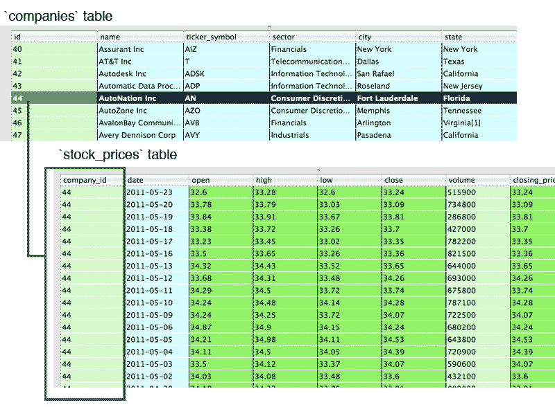
With a database, we can reduce this redundancy by creating two tables: one for the company information and one for the company stock performance. The relationship between company and stock price records is a many-to-one relationship: One company has many stock price records.
Unique keys
In the stock_prices table, how do we know which records belong to which company? We need a column in stock_prices that refers to the company of each record. In other words, some kind of identifying value unique to each company that can be matched against a column in companies.name.
An obvious identifier would be the value in companies.name or in companies.ticker_symbol, assuming no two companies share the same value:
However, this results in the problem of having companies.name being repeatedly needlessly inside of the stock_prices table. This can be avoided by creating a new column – typically called 'id' for the companies table and a corresponding stock_prices.company_id column.
Again, think of the real-world implications. If we use companies.name as a unique identifier, we have to change that value as well as all the corresponding stock_prices.company_name values. But by giving each company an arbitrary id value – which can be a simple integer – the only thing each row in stock_prices has to worry about is that it has the right id value, which (ideally) should never change, no matter what identity crisis a company may undergo.
The JOIN and ON syntax
OK, back to SQL code. Now that we've split our data into two tables, we need to use a JOIN keyword to return rows that contain fields from both tables. The following returns all rows with the company and stock price info (thus, pretty much what we could do with SELECT * from companies_and_stocks previously):
SELECT companies.*, stock_prices.*
   FROM companies
   INNER JOIN stock_prices
      ON stock_prices.company_id = companies.id
   WHERE stock_prices.closing_price > 100
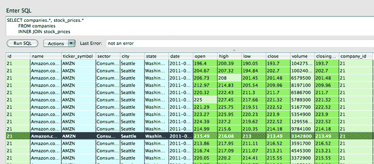
Let's break the syntax down:
- SELECT companies.*, stock_prices.*
- Because we want every column from each table, we have to explicitly refer to each table in the SELECT keyword.
- FROM companies
- This is slightly confusing because in the SELECT, we referred to another table, stock_prices. However, the SELECT only specifies what columns we want to return, regardless if its from the FROM-specified table or not. Specifying companies here only defines a starting set of data to join other tables onto.
- INNER JOIN stock_prices
- There are other kinds of joins, but INNER JOIN is one of the more commonly-used, and is useful for our purpose. The inner join will return one record for every combination of row in the left side and row in the right side. So, an INNER JOIN without any kind of conditional operators (used in ON) will return the number of rows equal to the number of rows in companies multiplied by the number of rows in stock_prices.
- ON stock_prices.company_id = companies.id
-
You can try running the query without the ON clause, but it will probably crash your program.
The result is a massive table (again, number of companies rows * number of stock_prices row) of nonsensical data, because the INNER JOIN returns every combination of company and stock price record, whether the record belongs to the company or not.
In fact, running this query: SELECT COUNT(1) FROM companies INNER JOIN stock_prices will result in 228,389,500 records (the product of 500 companies times 450,000+ stock price records)
The ON keyword is used to specify a condition for those matches. We don't want every combination of company and stock price. We only want the combinations in which stock_prices.company_id = companies.id. As with WHERE, you can use a long series of boolean and logical operators as conditions.
- WHERE stock_prices.closing_price > 100
-
The WHERE keyword, as we've been using it, comes after the JOIN and ON keywords.
It may seem that you can put the condition used in WHERE inside the ON keyword. This often works fine (I can't say I've tried all the possibilities). But the general rule is:
- Use ON to constrain the relationships between joined tables.
- Use WHERE to limit the records returned overall.
This makes particular sense in cases where there are multiple tables joined together. For example:
SELECT * FROM t1
   INNER JOIN t2 ON t1.id = t2.xid
   INNER JOIN t3 ON t2.id = t3.yid
Subqueries
Just in case you thought that JOIN clauses didn't make a SELECT statement busy enough: Subqueries allow you to pull in a derived table or datapoint using a separate query.
They are sometimes referred to as nested queries, as they are queries inside another (main, or "outer") query.
Let's say we want to find the result set with all the columns from the companies table, plus the closing price for each company on the most recent date in the stock_prices table.
Let's first look at how you would find the latest closing price for just the company with id of 1:
SELECT company_id, date, closing_price FROM stock_prices WHERE company_id = 1 ORDER BY date DESC LIMIT 1
Using a subquery, we can run that query for every company in companies:
SELECT companies.*,
    (SELECT closing_price FROM stock_prices
         WHERE companies.id = company_id
         ORDER BY date DESC LIMIT 1 ) AS latest_closing_price
    FROM companies
In this example, we are using the subquery to pull in a single datapoint – the latest closing_price where stock_prices.company_id = companies_id. I use LIMIT 1 to explicitly limit the subquery result to 1 result row. SQLite appears to take the top row by default, but other flavors of SQL may raise an error if the subquery has more than one result.
However, the subquery must return only one column.
Alias the subquery result
It is useful – but not necessary – to alias the subquery. You can use the alias in a subsequent WHERE clause:
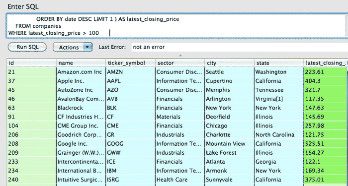
SELECT companies.*,
    (SELECT closing_price FROM stock_prices
      WHERE companies.id = company_id
      ORDER BY date DESC LIMIT 1 ) AS latest_closing_price
    FROM companies
WHERE latest_closing_price > 100
The result:
Bonus question: What's the difference between having the closing_price > 100 condition in the subquery versus having it as a condition in the main query, i.e. WHERE latest_closing_price > 100?
Answer: In the subquery, that condition will find the latest closing_price that was above 100. In the main query, this condition only returns companies in which their most recent closing_price was above 100. The latter group is equal to or smaller than the former group, as many companies may have had a closing_price above 100 throughout the timespan covered in stock_prices.
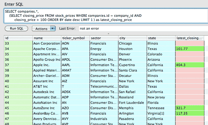
In fact, using the closing_price condition in the subquery will return a result set of every company, though some of them will have no value for latest_closing_price if none of their stock price records had a closing_price > 100. Try it yourself:
SELECT companies.*,
    (SELECT closing_price FROM stock_prices WHERE companies.id = company_id
      AND closing_price > 100
      ORDER BY date desc LIMIT 1 ) as latest_closing_price
FROM companies
The result:
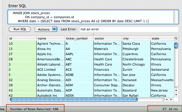
Using a subquery in the WHERE clause
Subqueries can be executed outside of the SELECT clause of a query. In the following, I've put it in the WHERE clause:
SELECT companies.*,  closing_price AS latest_closing_price
    FROM companies
    INNER JOIN stock_prices
      ON company_id = companies.id
    WHERE date = (SELECT date FROM stock_prices AS s2 ORDER BY date DESC LIMIT 1 )
The table below compares two versions of the same query: when the subquery is in the WHERE clause (as shown in the example immediately above) to the previous version of this query, where the subquery was part of the main query's SELECT clause:
| SUB1: Subquery in main SELECT clause | SUB2: Subquery in WHERE clause |
|---|---|
SELECT companies.*,
   (SELECT closing_price FROM stock_prices
      WHERE companies.id = company_id
      ORDER BY date DESC LIMIT 1 )
      AS latest_closing_price
      FROM companies
|
SELECT companies.*,  closing_price AS latest_closing_price
   FROM companies
   INNER JOIN stock_prices
   ON company_id = companies.id
    WHERE date = (SELECT date
      FROM stock_prices
AS s2 ORDER BY date DESC LIMIT 1 ) |
|
Number of times subquery executes: Once for each company row |
Number of times subquery executes: Just once |
|
Execution speed (on my laptop): 1,500 milliseconds |
Execution speed (on my laptop): 15-30 milliseconds |
There is one very important distinction, however: In the version in which the subquery is in the WHERE clause (SUB2), the subquery executes only once. Hence, it only finds a single latest date with which to filter the results by.
Therefore, if a given company does not have a record for that date, it won't show up in the main query's results. So SUB2 returns only 496 companies instead of the expected 500 that SUB1 returns.
Beyond SELECT
This chapter only covers a subset of SQL commands relating to retrieving records. We did not cover the syntax for creating tables, inserting records, updating and deleting records.
Nor did we cover the concept of creating indexes for tables, which is necessary for speedy SELECT statements (in the sample data, I've indexed the tables for you).
But you know enough about the structure of SQL concepts to grok the SQLite manual yourself. In the Common Surgeries project, I include a walkthrough of these SQL operations.
I also have done a quick writeup, with code, demonstrating how I gathered the stock listings and created the SQLite database.
Using SQLite3 with Ruby
So far we've been writing pure SQL, which is pretty powerful on it's own. But if you're like me, SQL's syntax seems more opaque than scripting languages such as Ruby and Python.
When SQL queries involve subqueries and joins, the syntax can get especially difficult. With Ruby, though, we can use the constructs we already know – such as loops and collections – and combine them with SQL calls to do a wide range of powerful data-crunching techniques.
The sqlite3 gem
At the beginning of this chapter, you installed the SQLite3 software. To get it to play with Ruby, you need to install the sqlite3 gem:
gem install sqlite3
The have been a few problems reported on getting this gem to install. I wish there were a cure-all, but the solution to whatever problem you might have is dependent on how you installed SQLite (was it pre-installed? Did you use Homebrew (Mac OS X)?). Again, searching the Internet is your best bet.
Test out the sqlite3 gem
Once you've installed the gem, try out the script below. It simply creates a new database file named "hello.sqlite" and then executes the following SQL operations:
- CREATE a table named testdata with columns class_name and method_name
- INSERT a bunch of rows
- And several SELECT statements: number of entries, the 20 longest method names, and the 10 most common method names
The results from the SQL SELECT statement will be stored as a Ruby array and then iterated through
require 'rubygems'
require 'sqlite3'


DBNAME = "hello.sqlite"
File.delete(DBNAME) if File.exists?DBNAME

DB = SQLite3::Database.new( DBNAME )
DB.execute("CREATE TABLE testdata(class_name, method_name)")

# Looping through some Ruby data classes

# This is the same insert query we'll use for each insert statement
insert_query = "INSERT INTO testdata(class_name, method_name) VALUES(?, ?)"

[Numeric, String, Array, IO, Kernel, SQLite3, NilClass, MatchData].each do |klass|
  puts "Inserting methods for #{klass}"

  # a second loop: iterate through each method
  klass.methods.each do |method_name|
    # Note: method_name is actually a Symbol, so we need to convert it to a String
    # via .to_s
    DB.execute(insert_query, klass.to_s, method_name.to_s)
  end
end


## Select record count
q = "SELECT COUNT(1) FROM testdata"
results = DB.execute(q)
puts "\n\nThere are #{results} total entries\n"

## Select 20 longest method names
puts "Longest method names:"
q = "SELECT * FROM testdata
ORDER BY LENGTH(method_name)
DESC LIMIT 20"
results = DB.execute(q)

# iterate
results.each do |row|
  puts row.join('.')
end


## Select most common methods
puts "\nMost common method names:"
q = "SELECT method_name, COUNT(1) AS mcount FROM testdata GROUP BY method_name ORDER BY mcount DESC, LENGTH(method_name) DESC LIMIT 10"
results = DB.execute(q)
# iterate
results.each do |row|
  puts row.join(": ")
end
This is the sample output:
There are 715 total entries
Longest method names:
Numeric.instance_variable_defined?
Numeric.protected_instance_methods
String.instance_variable_defined?
String.protected_instance_methods
Array.instance_variable_defined?
Array.protected_instance_methods
# ...
If you open up the file using the Firefox SQLite Manager (whereever the script saved hello.sqlite), the testdata table looks like this:
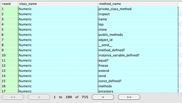
The next section will walk through some of the basic functionality of the sqlite3 gem. The rest of this chapter will work off of the database of Standard & Poor's 500 stock listings. Save the .sqlite file to whatever directory in which you are testing out your Ruby + sqlite3 gem scripts.
Opening up a database
require 'rubygems'
require 'sqlite3'
db = SQLite3::Database.new('sp500-data.sqlite')
The first step is to require the sqlite3 library. Then we create a handle for a database file with the SQLite3::Database.new method.
If the file doesn't exist, a new SQLite database is created.
EXECUTE
results = db.execute("SELECT * from companies;")The execute method is the basic way of doing single queries in Ruby. In the chapter so far, we haven't had the need to do more than one statement at once. However, you'll find yourself wanting to write multiple queries in a single string when doing INSERT or UPDATE operations. The SQLite3 docs describe the execute_batch method.
Query results
In the above exercise, what form does the return value of db.execute come in?
require 'rubygems'
require 'sqlite3'
db = SQLite3::Database.new('sp500-data.sqlite')
results = db.execute("SELECT * FROM companies where name LIKE 'C%'")
puts results.class
#=> Array
The results come as an Array, which means you can iterate through them like any collection:
results.each{|row| puts row.join(',')}72,C. H. Robinson Worldwide,CHRW,Industrials,Eden Prairie,Minnesota 73,CA, Inc.,CA,Information Technology,Islandia,New York 74,Cablevision Systems Corp.,CVC,Consumer Discretionary,Bethpage,New York 75,Cabot Oil & Gas,COG,Energy,Houston,Texas 76,Cameron International Corp.,CAM,Energy,Houston,Texas 77,Campbell Soup,CPB,Consumer Staples,Camden,New Jersey 78,Capital One Financial,COF,Financials,Tysons Corner,Virginia 79,Cardinal Health Inc.,CAH,Health Care,Dublin,Ohio
Each entry in the array is itself an array, with elements for each column of the query. So think of the returned results as a table, in which each row is in the main array:
puts results[2].join(', ')
#=> 74, Cablevision Systems Corp., CVC, Consumer Discretionary, Bethpage, New York
And each row contains an array of columns:
puts results[2][1]
#=> Cablevision Systems Corp.
Access the columns by column name
If your SELECT query returns a lot of columns, you'll probably find it easier to refer to the columns by name rather than numerical index. You can do this with the SQLite gem by changing a property on the database:
db.results_as_hash = trueNow each row will act as a Hash; note that you have to change the setting before executing the query:
require 'rubygems'
require 'sqlite3'
db = SQLite3::Database.new('sp500-data.sqlite')
db.results_as_hash = true
results = db.execute("SELECT * FROM companies where name LIKE 'C%'")

puts results[0].class
#=> Hash

puts "#{results[0]['name']} is based in #{results[0]['city']}, #{results[0]['state']}"
#=> C. H. Robinson Worldwide is based in Eden Prairie, Minnesota
Exercise: Filter results with select
In the earlier discussion on subqueries, we examined a query that attempted to find the latest stock price per company.
This time, instead of using subqueries, write two SQL queries and combine it with Ruby looping logic. Remember that subqueries can be thought of as "inner queries" to be executed before the query in which they are nested.
Write the Ruby code that will perform the following query without subqueries:
SELECT companies.*,  closing_price AS latest_closing_price
   FROM companies
   INNER JOIN stock_prices
      ON company_id = companies.id
    WHERE date = (SELECT date FROM stock_prices AS s2 ORDER BY date DESC LIMIT 1 )
Solution
require 'rubygems'
require 'sqlite3'
db = SQLite3::Database.new('sp500-data.sqlite')
db.results_as_hash = true

inner_results = db.execute("SELECT date FROM stock_prices ORDER BY date DESC LIMIT 1")
latest_date = inner_results[0]['date']

results = db.execute("
SELECT companies.*,  closing_price AS latest_closing_price
   FROM companies
   INNER JOIN stock_prices
      ON company_id = companies.id
    WHERE date ='#{latest_date}'
")

results.each{|row| puts "#{row['name']}: #{row['latest_closing_price']} "}
The results:
Agilent Technologies Inc: 40.89
Alcoa Inc: 11.57
Apple Inc.: 404.95
AmerisourceBergen Corp: 42.08
Abbott Laboratories: 54.22
...
Zions Bancorp: 18.24
Zimmer Holdings: 54.3
Placeholders
The SQLite3 gem has a nifty feature that takes care of the quotes and escaping backslashes for us. Let's say we have a program that has an array of city names:
city_names = ["New York", "Coeur d'Alene", "Boise"]And then the program loops through each city name and runs this query:
db.execute("SELECT * FROM companies WHERE city LIKE '#{city_name}%'")
There's a slight problem here, though. When city_name is "Coeur d'Alene", the program will attempt to execute the following query:
db.execute("SELECT * FROM companies WHERE city LIKE 'Coeur d'Alene%'")
Do you see the error? It's caused by the city name having an apostrophe, which prematurely closes the string in the SQL query. It's easy to fix this by rewriting the code, like so:
db.execute("SELECT * FROM companies WHERE city LIKE \"Coeur d'Alene\%"")
But in a program with more complicated queries, this is a pain to do. Thankfully, we can have the SQLite gem do the work for us by using placeholders in the query and then passing extra values to the execute method:
city_names = ["New York", "Coeur d'Alene", "Boise"]
city_names.each do |city_name|
   res = db.execute("SELECT * FROM companies WHERE city LIKE ?", "#{city_name}%")
   puts "Number of companies in #{city_name}: #{res.length}"
end
- The question mark ? is used as a placeholder
- The number of extra arguments must match the number of placeholders. In the above example, there is one place holder, thus, one extra argument.
- If there are multiple placeholders, the extra arguments are inserted in order, left to right.
The main thing is to make sure your number of arguments match the number of placeholders and to keep them in the correct order.
Exercise: Find stock prices within a random range
Write a program that:
- Generates two random numbers, x and y, with y being greater than x. Both numbers should be between 10 and 200.
- Executes a query to find all stock_prices in which the closing_price is between x and y
- Outputs the number of stock_prices that meet the above condition
- Does this operation 10 times
Solution
require 'rubygems'
require 'sqlite3'
db = SQLite3::Database.new('sp500-data.sqlite')

10.times do
   x = rand(190) + 10
   y = x + rand(200-x)
   res = db.execute("SELECT COUNT(1) from stock_prices WHERE closing_price > ? AND closing_price < ?", x, y)
   puts "There are #{res} records with closing prices between #{x} and #{y}"
end
Sample output:
There are 4639 records with closing prices between 125 and 164
There are 12795 records with closing prices between 101 and 193
There are 23304 records with closing prices between 51 and 56
There are 306415 records with closing prices between 24 and 112
There are 125928 records with closing prices between 46 and 100
There are 29776 records with closing prices between 74 and 109
There are 157 records with closing prices between 195 and 199
There are 270 records with closing prices between 174 and 180
There are 1792 records with closing prices between 133 and 148
There are 6290 records with closing prices between 120 and 171
Using an array with placeholders
The execute method will accept an array as an argument, which it will automatically break apart into individual arguments. So of course, the number of elements in the array must match the number of placeholders:
db.execute("SELECT * from table_x where name = ? AND age = ? and date = ?, ['Dan', 22, '2006-10-31'])Exercise: Find all company names that begin with a random set of letters
Write a program that:
- Generates a random number, from 1 to 10, of random alphabetical letters.
- Executes a query to find all the company names that begin with any of the set of random letters
- Outputs the number of companies that meet the above condition
- Does this operation 10 times
The main difference between this exercise and the previous one is that you don't know how many placeholders you'll need for the query. You can use string interpolation and Enumerable methods to dynamically generate the placeholders.
Hint: You can generate an array of alphabet letters with this Range:
letters = ('A'..'Z').to_a
Solution
You don't have to use interpolation since we're only dealing with single letters with no chance of apostrophes. But this is practice:
require 'rubygems'
require 'sqlite3'
db = SQLite3::Database.new('sp500-data.sqlite')

LETTERS = ('A'..'Z').to_a

10.times do
   random_letters = LETTERS.shuffle.first(rand(10) + 1)
   q = random_letters.map{"name LIKE ?"}.join(' OR ')
   res = db.execute("SELECT COUNT(1) from companies WHERE #{q}", random_letters.map{|r| "#{r}%"})
   puts "There are #{res} companies with names that begin with #{random_letters.sort.join(', ')}"
end
Sample results:
There are 186 companies with names that begin with C, G, M, P, T, W, Y, Z
There are 219 companies with names that begin with B, C, H, I, M, N, S, V, Z
There are 185 companies with names that begin with C, M, N, O, Q, S, T
There are 104 companies with names that begin with C, O, P, U
There are 14 companies with names that begin with R
There are 74 companies with names that begin with B, M, Q, R
There are 109 companies with names that begin with E, F, M, T, X, Y
There are 189 companies with names that begin with B, C, E, F, H, I, O, R, V, Y
There are 191 companies with names that begin with A, G, H, I, M, N, Q, V, W, Z
There are 28 companies with names that begin with J, W
Take it slow
If you're just learning Ruby, then having to figure out another completely different syntax – SQL – is going to be difficult. So don't feel overwhelmed; this is supposed to be a little complicated.
My main purpose was to introduce you to the concepts and demonstrate their use in day-to-day programming. So when you get comfortable with Ruby and have a few data-intensive programs in mind, you'll at least know where to start.
I never learned SQL formally because I didn't think I wanted to be a database programmer. And I still don't. I only learned the SQL I know by looking up references and asking for help. You'll find that once you know a concept exists – whether it is SQL or anything – you'll pick it up quickly when you need to actually use it.
Many of the projects in this book (will) use databases simply as a fast way to store and access information; you can learn by example from the projects. And Artful Software's Common MySQL Queries page is a gold mine of examples.